Table of Contents
Introduction
This tutorial will guide the user through the steps required to run all the components of the Cartesian Interface with the purpose of controlling a generic yarp-compatible robot limb in its operational space. Therefore, this is a somewhat advanced topic which might be of interest just for developers who want to adopt this interface for their platforms, or for those of you who are really geek inside :).
For "normal" people - who have only iCub in their work life - the tutorial on the Cartesian Interface is extensive enough; it is also a prerequisite for proceeding further.
The Architecture
The architecture of the Cartesian Interface is sketched out below.
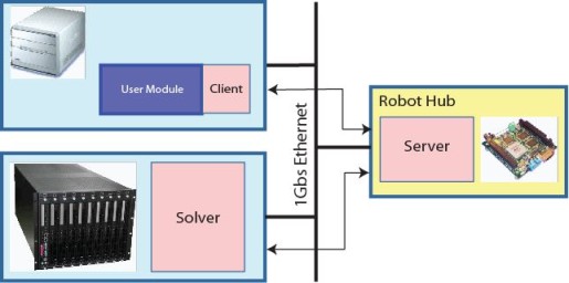
We already know there is a solver in charge of inverting the kinematics, a server controlling the robot limb and finally a client enabling the user to forward requests for cartesian movements directly from within the code through typical calls to C++ methods.
However, the diagram is more informative than that: it tells us about how these three components are arranged in the iCub network, an allocation that should be preserved also for your robot's architecture to achieve fast and reliable performances. Here follow the details.
- The solver is the most computational demanding tool; for this reason it should be launched on a powerful machine belonging to the cluster of PCs connected to the robot network. It employs Ipopt for nonlinear optimization and should not be a burden to any critical routine that has to control the robot in real-time.
Nonetheless, running on a powerful computer, the solver can tackle the inverse kinematics problem with a large number of degrees-of-freedom in near real-time (something like ~30 ms). This level of performance lets the robot do tracking pretty nicely. - The server is a canonical controller responsible for sending commands to the robot with the purpose of achieving the joints configuration as found by the solver by moving the limb in a human-like fashion. It is a light-weight program so that it can run directly onboard the robot hub; it collects the requests coming from all the clients, it asks the solver to do its job and feeds back clients with useful information such as the current end-effector pose.
The main reason why the server should be running on the hub is that the lag due to the communication must be reduced as much as possible since a lag in the control loop will inevitably cause for instance unwanted overshoots in the response. As final suggestion, consider placing the server physically close to the robot, that is where fast ethernet link ends (and yarp too) and the internal robot bus begins (e.g. CAN); for iCub indeed, the server runs aboard the icub-head. - The client simply lives inside the user code, making queries to the server through yarp ports, thus it never speaks to the solver. There are no special needs for it: the location of the client depends only on the requirements of the user code; a program that opens up a client may run on a shuffle PC so as on a powerful machine or even aboard the robot hub.
Dependencies
Besides the "classical" dependecies you need to have in order to compile all the components (Ipopt, yarp, icub-main, iKin, servercartesiancontroller, clientcartesiancontroller; you should know them very well by now :), you are required to accomplish a preliminary job: it can be tedious (I realize it when I had to write the "fake" stuff :) but is mandatory. You have to provide some low-level yarp motor interfaces that are necessary for the cartesian components to start and operate correctly. They are only three: IControlLimits, IEncoders, IVelocityControl. The former two serve to get the number of joints, their actual range along with current joints configuration which is fed back to the controller; the latter is obviously employed to send velocity commands to the robot.
Alternatively, user might consider implementing the newest IEncodersTimed motor interface in place of IEncoders, providing also information about the time stamps of the encoders that in turn will be attached to the pose information for synchronization purpose. At startup, the cartesian server will check accordingly the availability of the most suitable encoders interface.
Moreover, as enhanced option, the server is also capable of automatically detecting the availability of the IPositionDirect interface, through which the low-level velocity control is replaced by the faster and more accurate streaming position control. In this latter modality, also the standard IPositionControl interface is required to be implemented.
This is not the right place where to tell about how to deal with these interfaces, but please find out more on the topic of making a new device in yarp.
Example of Customization
Let's explain how to configure all the components for your robot through an example, whose code is available under
Imagine you're done with coding the basic motor interfaces for your robot, which is not as cute as iCub: it is equipped indeed with just three degrees-of-freedom represented by three joints controlled by three independent motors. You'll probably end up having something similar to the library fakeMotorDevice I wrote for our artifact. It contains the server and client implementations of such motor interfaces: again, the IControlLimits, the IEncoders and the IVelocityControl. Of course we would need now a program that simulates our fake manipulator together with the server layer that exposes a yarp access to it. Here it is: it's called fakeRobot and instantiates three motors that are embodied as pure integrators that give back joints positions once fed with joints velocities.
The relevant code snippet of this instantiation is located within the file fakeMotorDeviceServer.cpp and resumed here for your convenience:
Aside from the details of the Integrator class (it is provided by the ctrlLib library), it is worth noticing here how the joints have bounds defined by the matrix lim.
Now, since you're so motivated, you've already got the kinematic description of the manipulator from your colleague who's hooked on mechanics. You have to provide the conventional Denavit-Hartenberg table of links properties as done for the fake robot in the file app/conf/kinematics.ini:
The meaning of these parameters is described in the iKinLink class; at any rate they are easily recognized as the link length (A in [m]), the link offset (D in [m]), the link twist (alpha in [rad]) and so on: please visit the documentation on kinematics for a deeper insight.
A careful reader should have not missed the expression for the joints limits, which here can definitely take whatever values for all the three joints, much different from the bounds assigned to the real joints and hard-coded within the fake motor device. Do not worry about that: at start-up the solver will query the low-level interface (namely IControlLimits) about the actual joints range and will update the kinematic structure accordingly. Later on, the server will get upgraded with a similar request to the solver.
At this stage we are happy with the kinematics, so let's continue with the components configuration.
Configuring the Solver
What is required here is only to inherit a new class from the iKin superclass CartesianSolver and then override the method getPartDesc() which is responsible for describing all the parts used by the solver.
Essentially, you have to do the following four things:
- Retrieve the configuration parameters;
- Initialize the devices to access the motors;
- Retrieve information about the kinematics;
- Fill a descriptor to be returned to the superclass.
1. Retrieving Configuration Parameters
The parameter of the getPartDesc() method is a Searchable object that should contain the initial configuration of the solver as provided for instance through the file solver.ini whose content is listed just below. However, these values can be easily modified at run-time through calls to the cartesian interface methods.
2. Initializing Motor Devices
The solver must be aware of how to open a client to speak to motor device drivers. Prepare therefore as many Property objects containing the suitable options as it is required by the manipulator: i.e. if the manipulator is composed of two parts (e.g. torso + arm), prepare one Property for each part, filled with the instructions to open the corresponding motor client.
In the current example the fake manipulator is represented by just one motor part as it follows:
3. Retrieving Kinematics Info
There is a special key in the configuration file solver.ini which is missing: the one that tells the solver how to retrieve the kinematics description. Its tag is "CustomKinFile" and must point to the kinematics.ini file. The path has to be absolute and can be easily completed automatically by the ResourceFinder class - as you know: that's why we code it like the following:
We then build up the kinematic structure by populating an iKinLimb object with such information:
4. Filling the Descriptor
Finally, we need to provide a descriptor that in turn will be processed by the superclass:
(*) It may happen that the motor commands to be sent are in reversed order with respect to the order of kinematics links as in the case of the iCub torso; if so, push a "true" in the rvs field for the corresponding part.
Whenever a limb is actuated resorting to more than one device (e.g. for iCub: torso+arm), the following applies:
Intuitively, the insertion order depends on the links of the chain. In iCub the three links of torso come first, hence optTorso is the first object to be pushed in the queue.
To conclude, it is worth pointing out how all the steps described above can be conveniently handled also by means of the iKinCartesianSolver module.
Configuring the Server
Coming to the server, life gets a bit easier. It is indeed required to open the device drivers of each involved part (in our case just one, the "fake_part"), put them into a special list, open the cartesiancontrollerserver device passing the proper configuration parameters that ensure the initialization of the kinematic structure, finally attach that list to such cartesian device.
The code is worth a thousand words ...
The configuration parameters of the server are the following:
(*) When "on" this parameter enables the low-level streaming position control of the robot's joints, meaning that the server will provide as output the position set-points straightaway instead of the velocity commands. As result, we gain much faster and more accurate movements, without requiring any ad-hoc dynamics compensation (see below). To do that, the IPositionDirect interface needs to be available.
(**) When "on" allows sending references to multiple joints with one yarp command saving bandwidth; when "off" each yarp command carries reference for one single joint.
(***) This is an optional parameter that accounts joint by joint for the minimum velocity (in [deg/s]) the motors can somehow achieve, and are meant to be provided in absolute values. Whenever the controller tries to deliver velocities under these thresholds, then it switches in a bang-bang mode to finally attain the target positions.
Plant Identification (Advanced)
This topic is somewhat advanced and is concerned with the possibility to improve the controller's performance, so that it is not strictly required for normal operations and the user might consider skipping it at the early stage of his implementation. Further, if the IPositionDirect interface is detected as available by the server and the PositionControl configuration switch is set to "on", then the presence of the section [PLANT_MODEL] described hereinafter will turn to be irrilevant to the control.
The closed-loop joint controller is designed in such a way that it delivers velocity commands to shape the system response as to follow a trajectory that resembles a minimum-jerk profile. To this end, the strong assumption is that the joint itself behaves like a pure integrator. Of course the real world deviates - sometimes significantly - from the ideal conditions and a number of unmodelled factors starts taking place. In this respect, the following two elements deserve particular care since they can be conveniently compensated: (1) the high-order plant dynamics, (2) the dead-time affecting the plant response.
Regarding the high-order plant dynamics, as it is traditionally envisaged, a chirp signal can be injected into the system with the goal of identifying any further relevant zero and/or pole of the plant. Since the overall system is always stable and minimum-phase (i.e. both further poles and zeros belong to the left side of the complex plane), it derives that the controller is capable of filtering out the unwanted dynamics with pole-zero cancellation.
The framework can thus compensate plants characterized by the following transfer function:
\[ P\left(s\right)=\frac{K_p}{s}\cdot\frac{1+T_zs}{1+2\zeta T_ws+\left(T_ws\right)^2}\cdot e^{-T_ds}, \]
with two underdamped poles and one zero, besides the integrator. These parameters can be specified within the server configuration file for each joint belonging to the kinematic chain.
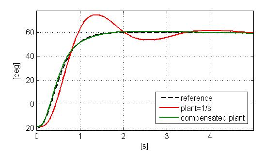
To give the feeling of how important could be accounting for this dynamics, take a look at the picture below, where the ideal response of a joint commanded by our velocity controller (dashed black) is depicted against the two real cases: with (green) and without (red) the compensation.
Interestingly, the application jointVelCtrlIdent available from this GitHub repository lets you collect information about the system response to the chirp command. You can then think of employing the System Identification Toolbox from MATLAB to find out where these unwanted poles and zero are located in the complex plane. In fact, the ident tool contained whithin the MATLAB package allows you to go through an identification session for the process P(s) specified above.
Finally, as very last step, one can try also to compensate the lag of the control system represented by the exponential term in the transfer function.
As you might know, a lag in a control loop is dangerous because it introduces distortions in the response. To recover the ideal response profile equalizing the lag, one common solution is to plug into the system a Smith Predictor. Nonetheless, this further block should be applied only when between the controller and the plant there exist significant and deterministic communication delays as it happens for example when the controller does not run on the robot hub.
Configuring the Client
The client does not have to be aware of any particular implementation, thus it can be configured as documented in the Cartesian Interface page. In this respect, to open a client that connects to server above one can rely on the following:
Compiling and Running the Example
The example has been designed according to the packaging policy we pursue for iCub-based application: there is a src directory filled with the library and the code and then there is an app directory containing the configuration files and the scripts to run the binaries. Therefore, just create the anyRobotCartesianInterface/build directory (be always neat and divide the code from the compilation products :), go there and launch the ccmake ../ command. After the compilation and the installation you'll end up having the directory anyRobotCartesianInterface/bin where all the binaries will be copied in, along with the configuration files and the xml scripts. Run the command yarprun --server /node from the same directory of the binaries and then launch in a row first the modules in robot_server_solver.xml and soon afterwards the modules in client.xml.
Success Stories
You are warmly encouraged to add up below your case study on the use of Cartesian Interface:
- Duarte Arag�o employed the Cartesian Interface for his robot Vizzy and documented the development here.
- Juan G. Victores managed to replicate the Cartesian Interface functionalities for Asibot whose server part is documented here.
- Elena Ceseracciu customized the Cartesian Solver for the ARMAR III robot. Relevant info can be browsed here.